Tag Archives: Data Collection

Data Collection – Boyle’s Law

Yesterday, as part of my Innovative Teaching Grant from the Pearland ISD Education Foundation, my students completed a data collection lab.

Objective

  • Model pressure versus volume using inverse variation

Procedure

Boyles Law Data Lab

Although students were in groups of three to four, each student collected their own data. Members of the group rotated between three jobs: syringe, calculator, directions.

A syringe containing 15 mL of air was screwed onto the gas pressure sensor, which was connected to the TI-Nspire.  The pressure of the air was recorded using the Data Quest App on the TI-Nspire.

Gas Pressure Sensor with Syringe

The gas was compressed to 14 mL, and the pressure was recorded.

Compressing the Air in the Syringe

The pressure reading was also recorded for 13 mL, 12 mL, 11 mL, and 10 mL.

Analysis

An example of one student’s data collection.

Pressure vs Volume Graph

Students noted that as the volume increased the pressure decreased.

The constant of variation was calculated by multiplying pressure and volume.  Then the average  was calculated.

Data Table

Using the mean value for the constant of variation, a model was written and graphed on the scatterplot of the data.

Inverse Variation Model

Results

Students used their models to predict the pressure for a volume of 20 mL and 5 mL.  Based on their predictions, they were able to determine that when the volume of a gas is decreased from 40 mL to 10 mL, the pressure will quadruple.

Data Collection – Exponential Part 2

Objectives

  • Record the successive maximum heights for a bouncing ball.
  • Model the bounce height data with an exponential function.

Procedure

Bounce Back

Groups of three students used a motion detector to collect the height of a bouncing ball for 5 seconds.

Ready to Bounce

Ready to Bounce

Bouncing Ball

Bouncing Ball

Analysis

An example of one group’s data collection.

Bounce Height Data Quest

Height vs Time Graph

Students determined the maximum height of five successive bounces.  They put the data in a List & Spreadsheets Page.

Bounce Height Data 1 Bounce Height Data 2

The data for the first and fourth bounce was used to mathematically determine an exponential model that would fit the data.  They plotted their data and model on a Data & Statistics Page.

Bounce Back Exponential

Calculated Model

Then they had the calculator find the exponential regression for their data.

Bounce Back Regression

Exponential Regression

Results

Most groups found their model and the exponential regression to be very similar.

Data Collection – Exponential

Today, as part of my Innovative Teaching Grant from the Pearland ISD Education Foundation, my students completed their third data collection lab.

Objectives

  • Record temperature versus time for a cooling object.
  • Model the temperature of an object as it cools.

Procedure

How Cool It Is

I had a crock pot of hot water.  Each group of three students were given a cup of the hot water.  They placed the temperature probe in the hot water for about 30 seconds, then removed the temperature probe and allowed it to cool.  The calculator collected the temperature data for three minutes.

probe in water

Temperature Probe in Hot Water

probe cooling

Temperature Probe Cooling

Analysis

An example of one group’s data collection.

Temp DataQuest before exp fit

Temperature vs Time Graph

Students determined that an exponential model should fit the data.  They had the calculator graph the exponential regression for their data.

Temp DataQuest

Temperature vs Time Graph with Exponential Regression

The exponential model did not appear to be a very good fit.  They determine that the exponential model should have an asymptote at room temperature.  So they adjusted the collected temperature values by subtracting the room temperature.  Then they sent the data to a Data & Statistics page for further analysis.

The data for 20 seconds and 160 seconds was used to mathematically determine an exponential model that would fit their adjusted temperature data.  They plotted their model, then compared their model to the exponential regression using the adjusted temperature data.

Temp with Plotted Function

Calculated Model

Temp with Regression

Exponential Regression

Results

Most groups found their model and the exponential regression to be very similar.

Data Collection – Inverse Variation

Objectives

  • Model pressure versus volume using inverse variation

Procedure

I had some extra time after reviewing for a test in one of my classes, so I got out the gas pressure sensor for us to model pressure versus volume. We had studied direct and inverse variation.

Since I only have two gas pressure sensors, we did this as a class demonstration using the TI-Navigator Live Presenter and one of the gas pressure sensors. One student had the calculator to capture the data and another student had the sensor with the syringe of air.

Most of my students are sophomores and are currently in Chemistry. They have not studied the gas laws, yet.  Before we started capturing the data, I had the student with the sensor increase and decrease the volume of air in the syringe. We looked at what was happening to the pressure and predicted that inverse variation would model the data.

Analysis

Pressure vs Volume Graph

Pressure vs Volume Graph

Pressure vs Volume Table

Pressure vs Volume Table

We looked at the table and saw that as the pressure increased, the volume decreased. We calculated the constant of variation by multiplying pressure and volume.

k Column

Constant of Variation Calculated Column

The constant of variation was relatively constant. The average was 20.4.

We plotted the inverse variation equation Inverse Variation Equation on our graph.

Pressure vs Volume Model

Inverse Variation Model

Data Collection – Quadratic

On Friday, as part of my Innovative Teaching Grant from the Pearland ISD Education Foundation, my students completed their second data collection lab.

Objectives

  • Record height versus time data for a bouncing ball.
  • Model a single bounce using both the vertex and standard forms of a parabola.

Procedure

That’s the Way the Ball Bounces Instructions

Since my subject partner’s classes were not participating in the data collection, we had ten CBR2 to share among all students in the class.  With several students out for a pep rally, students were able to work with a partner, and each student collected his/her own data.  Students dropped a racquetball below the CBR2 motion detector.  The CBR2 collected data for position vs time for 5 seconds.

Ball Bounce

Analysis

An example of one student’s data collection.

Bounce Data

Positive vs Time Graph

Students chose one bounce to model.  They selected the bounce and struck the outside data.

One Bounce

One Bounce

Then they sent the data to a Data & Statistic page to analyze the bounce.

Scatterplot of One Bounce

Scatterplot of One Bounce

They traced along the scatterplot to find the coordinates of the vertex.  They used the coordinates of the vertex to plot a function in vertex form.  Students had to change the value of a until they found the best fit for their data.

Scatterplot Vertex Form

Vertex Form

Then they expanded the vertex form to get the equation in standard form.  This student’s equation was Vertex to Standard Form.

Next they had the calculator find the quadratic regression for their bounce.

Scatterplot Regression

Quadratic Regression

Students compared the expanded vertex form equation to the standard form from the regression.  They found that the vertex form equation they had plotted was very similar to the standard form equation from the regression.

Students answered the questions on the record sheet.

That’s the Way the Ball Bounces Record Sheet

Conclusion

More than one student commented, “That was fun.”

Some of the juniors mentioned that they wished the had the TI-Nspire in Physics class.  They had recently done an experiment using the TI-84s with the motion detector to see how long it takes objects of differing masses to hit the ground.  They commented that it was easier to use the motion detector with the TI-Nspire.


Data Collection – Linear

On Wednesday, as part of my Innovative Teaching Grant from the Pearland ISD Education Foundation, my students and my subject partner’s students completed their first data collection lab.

Objectives

  • Model data using a linear equation.
  • Interpret the slope and intercept values from a linear model.

Procedure

Case 4 Flipping Coins Instructions

Due to larger than anticipated class sizes, time constraints, and limited 1982 pennies, students worked in groups of three to collect data for one set of pennies (pre-1982, 1982, or post-1982).  In a class of 30, four groups collected data for pre-1982 pennies, two groups collected data for 1982 pennies, and four groups collected data for post-1982 pennies.  After each group collected their data, the data was shared with the class and compared.

Data Lab

Results

Pre-1982

Pre-1982 Pennies

1982

1982 Pennies

Post-1982

Post-1982 Pennies

Students found that pre-1982 pennies were the most dense and post-1982 pennies were the least dense.  Based on their results, they determined that the composition of the penny changed in 1982.

Students interpreted the slope as the “weight” per penny and the y-intercept as the “weight” of the bucket.

For homework, the students completed the Case 4 Flipping Coins Evidence Record.

Case 4 Flipping Coins Evidence Record

Follow-up Questions

Today, I sent the students some follow-up questions using the TI-Nspire Navigator Quick Polls to assess their understanding.

I showed the students the graph below and asked “Which object weighs more?”.

follow-up graph

The results from one class period:

Q1

Almost every student correctly identified the correct answer.  All other periods had similar results.

Then I told the students, “The equation to model Object 1 is y = 0.5x + 0.5.  The equation to model Object 2 is y = 0.7x + 0.5”.  I asked, “What is the weight of the bucket?”.

The results from one class period:

Q2

Every student correctly input the correct answer.  All other periods had similar results.

Finally, to truly test their understanding of the meaning of the slope and y-intercept, I told the students, “You weighed 5 objects and found the weight to be 10 N.  The bucket weighed 0.5 N.”  I asked them to “Write an equation to model the weight of x objects.”.

The results from four class periods:

Q3     Q3

Q3     Q3

The first two classes needed some reteaching regarding slope.  The last two classes did better, but there is still room for improvement.  My last class period did not participate in the follow-up questions due to class orientation meetings during their class period.

Innovative Teaching Grant

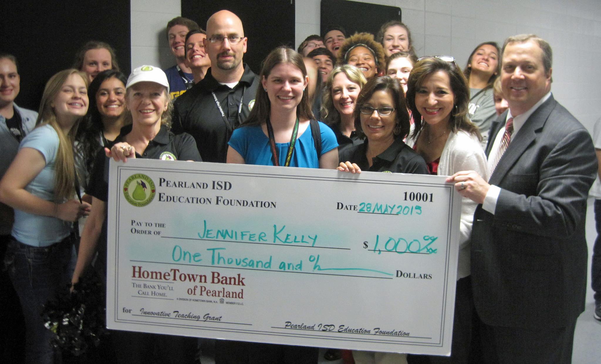
In March, I applied for an Innovation Teaching Grant through the Pearland ISD Education Foundation.  The project is described below.

Project Summary

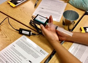
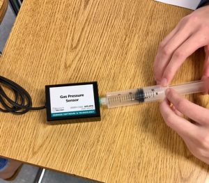
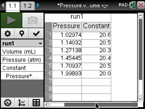
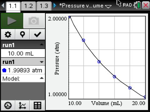
This project will provide the hardware required for real-time data collection by students working in small groups to support three Algebra 2 standards.  Real time data collection and analysis provides the tools to allow students to focus on the collected data and provides the foundation for application of the learning from the Algebra 2 curriculum to Science classes.

Purpose

There are three Algebra 2 standards that apply to data collection:
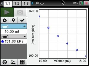
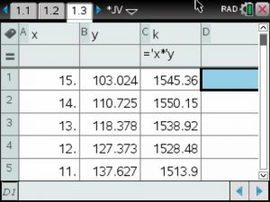
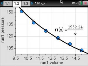
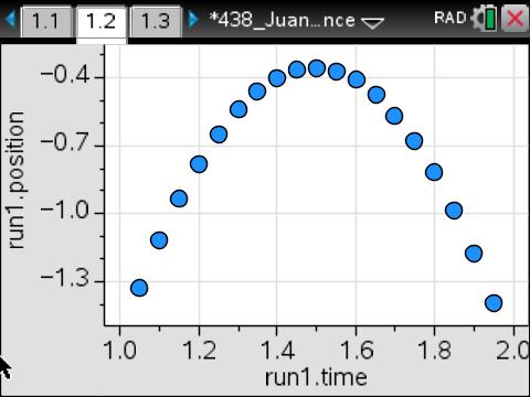
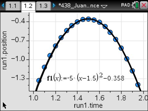
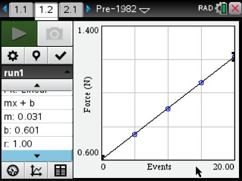
1.  Predict and make decisions and critical judgments from a given set of data using linear, quadratic, and exponential models.
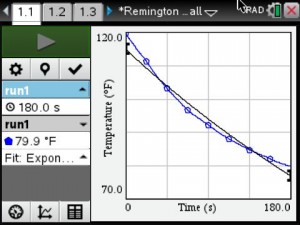
2.  Analyze data to select the appropriate model from among linear, quadratic, and exponential models.
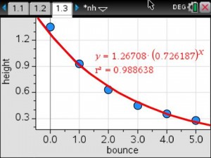
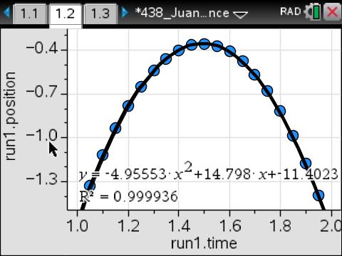
3.  Use regression methods available through technology to write a linear function, a quadratic function, and an exponential function from a given set of data.

The math department currently has a limited set of hardware which has been used for data collection to support these standards.  With limited equipment, the data collection must be performed by the teacher with the resulting data supplied to the students for analysis.

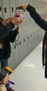
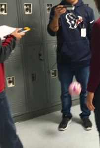
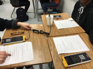
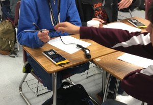
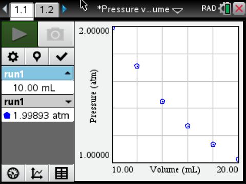
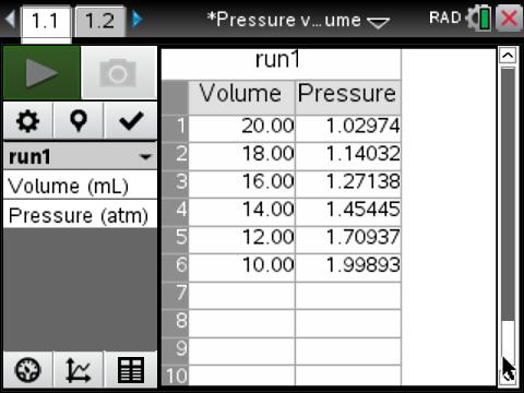
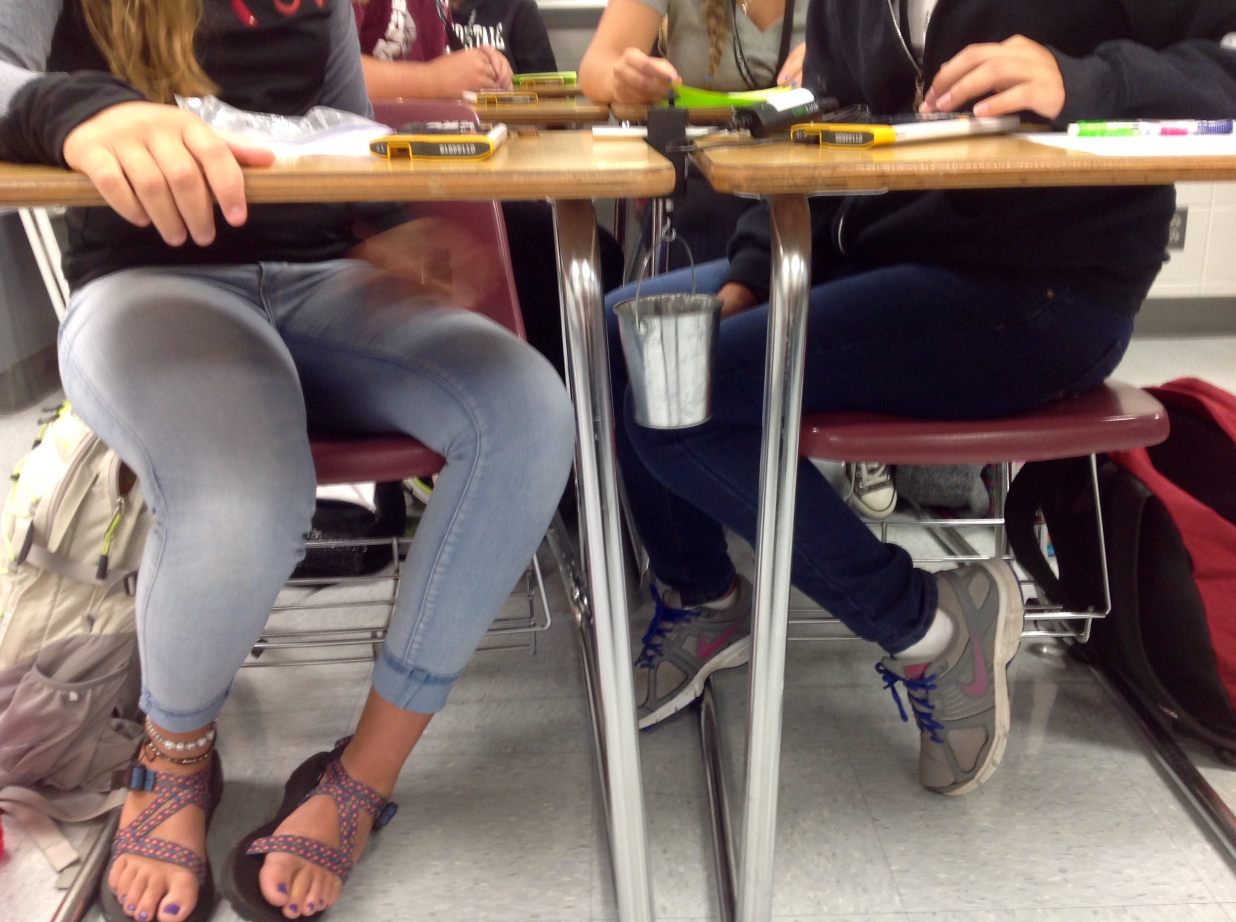
The purpose of the data collection project is to have students work in small groups to collect their own data, analyze and interpret the data, and predict and make decisions based on the appropriate model. In order for the students to perform the activities, we must have additional data collection equipment.

Objectives

By the end of the school year, all PAP Algebra 2 students will have completed at least three data collection activities (linear, quadratic, and exponential), working in small groups, utilizing the hardware supplied by this grant.

Project Description

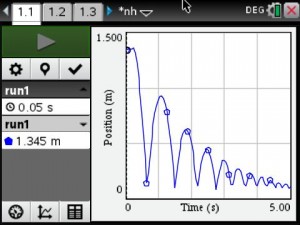
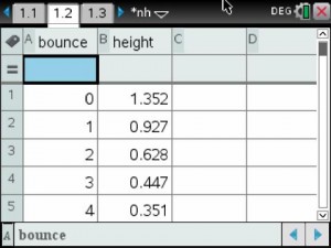
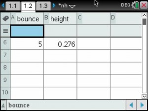
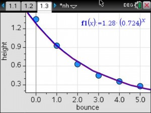
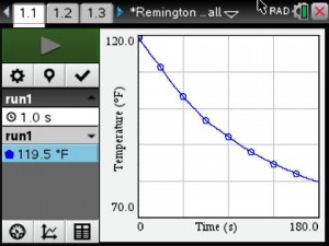
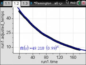
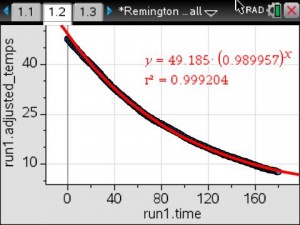
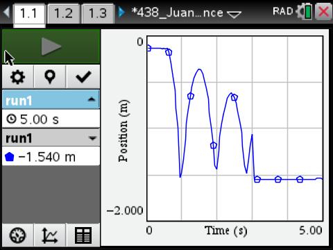
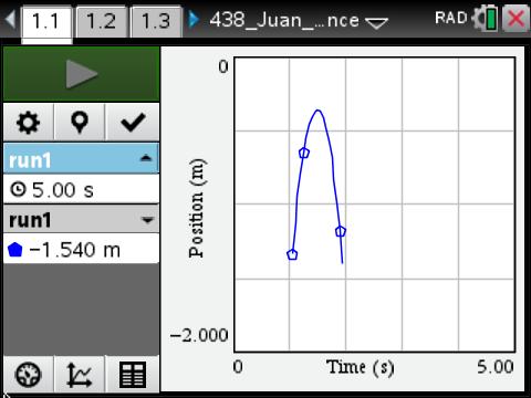
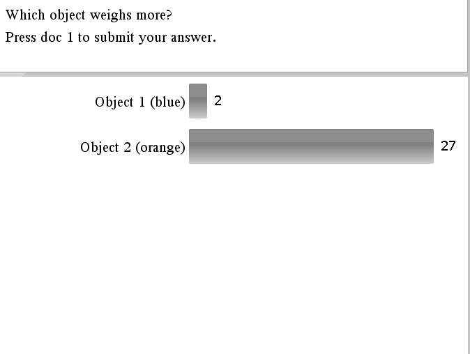
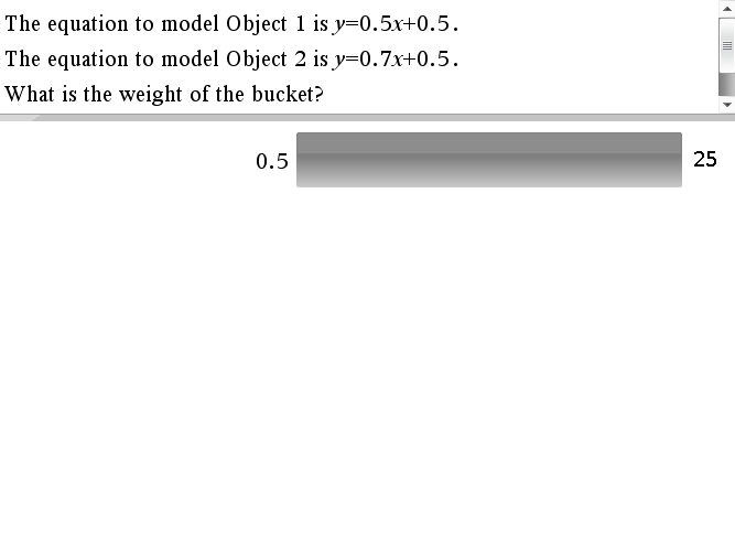
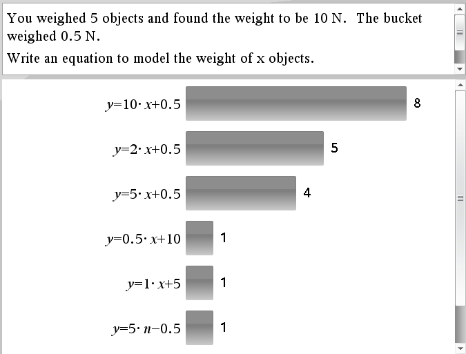
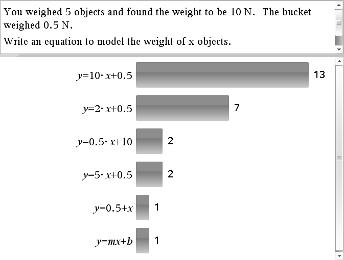
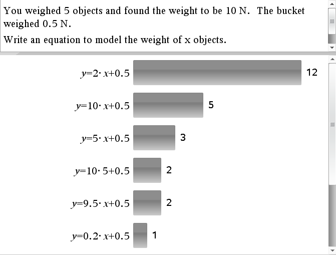
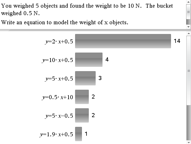
The teacher will use pre-made activities from TI’s Math Nspired or Vernier’s websites.  Possible activities include That’s the Way the Ball Bounces – Height and Time for a Bouncing Ball, Chill Out: How Hot Objects Cool, and Making Cents of Math: Linear Relationships between Weight and Quantity.

Research suggests that real-time data collection seems to be the most effective way to connect a graph with real-world experiences. (Lapp, Douglas A., and Vivian Flora Cyrus. “Connecting Research to Teaching: Using Data-Collection Devices to Enhance Students’ Understanding.” Mathematics Teacher 93.6 (2000): 504-10. – National Council of Teachers of Mathematics. Web. 28 Feb. 2015.)

Automated data collection improves the accuracy of the data collected and allows students to focus on the positive educational impact of the development of the mathematical model rather than the methodology of the data collection.

Real-time data collection by the students will supply the foundation for the application of linear, quadratic and exponential models to the analysis of physical measurements made in science curriculum.

Project Evaluation

Students will complete the student pages available through the pre-made activities.  The teacher will use the TI-Navigator to capture screen shots of the student’s data and to send quick polls to assess student’s understanding of concepts learned in each activity.

Budget

3 – Vernier EasyLink adapters – $175.50
3 – TI CBR2 motion sensors – $247.17
9 – Dual-range force sensors – $981.00

Other Funds Secured

For the students to perform their own data collection, working in small groups (4-5 students per group), there must be a total of 10 sets (5 sets per teacher) of data collection hardware.

The math department currently has:
2 – Vernier EasyLink adapters
2 – TI CBR2 motion sensors
6 – Temperature probes (5 personal property of one teacher)
1 – Dual-range force senors (personal property of one teacher)

Separate funding from a PTA grant has been secured for:
5 – Vernier EasyLink adapters – $292.50
5 – Temperature probes – $144.75
5 – TI CBR2 motion sensors – $411.95

Awarded May 28, 2015

grant